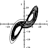
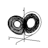
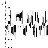
Lorenz's equation is one of the most tipical examples considered in the theory of ordinary differential equations. The first picture is the usual way of displaying the solutions: a projection to the (x,y) plane. The second picture is a 3 dimensional graphics of the solution. The third picture shows the x component of the solution as a function of t.


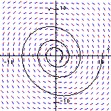
Another usual example is the damped pendulum. You can draw up the phase space with the direction field and the solution (first picture) and the energy function E=x*x+v*v (second picture). At the same time you can print out numerical values of t, x, v and E.
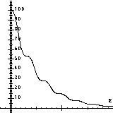
           t              x              v             E
        0.04000        9.99200       -0.39840       99.99879
        0.08000        9.96813       -0.79299       99.99253
        0.12000        9.92857       -1.18317       99.97632
        0.16000        9.87349       -1.56835       99.94545
        0.20000        9.80311       -1.94795       99.89540
        0.24000        9.71766       -2.32143       99.82188
        0.28000        9.61740       -2.68823       99.72088
        0.32000        9.50260       -3.04781       99.58864
        0.36000        9.37358       -3.39967       99.42172
        0.40000        9.23063       -3.74331       99.21698
        0.44000        9.07412       -4.07824       98.97160
        0.48000        8.90438       -4.40399       98.68313
        0.52000        8.72180       -4.72013       98.34943
        0.56000        8.52677       -5.02622       97.96875
        0.60000        8.31971       -5.32186       97.53969
        0.64000        8.10103       -5.60665       97.06121
        0.68000        7.87118       -5.88024       96.53266
        0.72000        7.63061       -6.14227       95.95371
        0.76000        7.37980       -6.39241       95.32444
        0.80000        7.11922       -6.63038       94.64526
        0.84000        6.84938       -6.85587       93.91692
        0.88000        6.57076       -7.06864       93.14051
        0.92000        6.28389       -7.26844       92.31745
        0.96000        5.98928       -7.45506       91.44945
        1.00000        5.68748       -7.62831       90.53854
        1.04000        5.37902       -7.78801       89.58700
        1.08000        5.06444       -7.93403       88.59737
        1.12000        4.74430       -8.06623       87.57244
        1.16000        4.41915       -8.18452       86.51518
        1.20000        4.08954       -8.28881       85.42878
        1.24000        3.75604       -8.37906       84.31658
        1.28000        3.41922       -8.45524       83.18208
        1.32000        3.07962       -8.51732       82.02889
        1.36000        2.73783       -8.56534       80.86070
        1.40000        2.39440       -8.59931       79.68128
        1.44000        2.04988       -8.61930       78.49444
        1.48000        1.70485       -8.62540       77.30401
        1.52000        1.35985       -8.61769       76.11381
        1.56000        1.01544       -8.59631       74.92762
        1.60000        0.67215       -8.56139       73.74919
        1.64000        0.33052       -8.51310       72.58216
        1.68000       -0.00890       -8.45163       71.43009
        1.72000       -0.34561       -8.37717       70.29641
        1.76000       -0.67908       -8.28995       69.18441
        1.80000       -1.00881       -8.19021       68.09721
        1.84000       -1.33430       -8.07821       67.03776
        1.88000       -1.65507       -7.95422       66.00882
        1.92000       -1.97064       -7.81854       65.01294
        1.96000       -2.28055       -7.67147       64.05243
        2.00000       -2.58436       -7.51335       63.12939
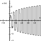
A functional differential equation can be solved and drawn just as easily. For example, the solution of the equation x'(t):=-a(t)*h(x(t))*x(t)-g(t,x(t-r(t))) (a, h, g and r are user defined functions) is shown on the next picture:
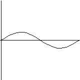
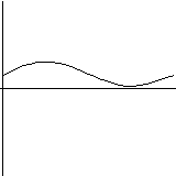
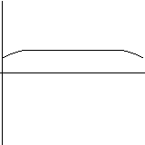
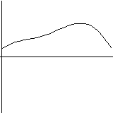
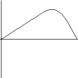
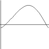
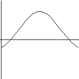
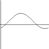
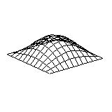
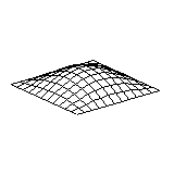
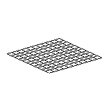
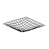
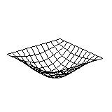
So far DifEqu has two kind of partial differential equations built in: PDE's on the line or PDE's on the plane. Mathematically it means that the unknown function depends on t and x or t, x and y, respectively. PDE's with more than two variables can also be programmed in DifEqu, I just did not have the time. Let us see the string with non-zero boundary conditions and the membrane with zero boundary conditions:

Of course, all of the above are just examples of the use of DifEqu, one can solve other equations, display it a different way or can write a program for solving an entirely different problem.
If this program seems to be suitable for your research, download this program to find it out.